Explain the methods, show your working and interpret results in context.
Foundation shows shared notes and questions. Higher includes the labelled extensions. Maps and checklist downloads include labelled Higher content; the worksheet generator filters individual goals.
Revise the key ideas
Time series and rates
Time-series display — Record the same measure at successive times and put time on the horizontal axis. Check equal time spacing and consistent definitions. A trend is the underlying longer-term direction; individual increases or decreases can reflect short-term noise or seasonality.
Seasonal and cyclic — Seasonal variation repeats on a fixed calendar cycle, such as higher summer sales each year. Cyclic variation repeats over longer or less fixed intervals, such as business cycles. Irregular variation includes unusual events; a single spike does not establish a seasonal pattern.
Four-point moving average — Average four successive values, then move one observation forward and repeat. For 10,14,18,22,30 the averages are 16 and 21. Plot each halfway between its middle two time points; use a common period length so regular seasonal changes are smoothed.Moving averages smooth a time series. Original illustrative diagram; numerical datasets are fictional worked examples.Enlarge diagram
Trend interpretation — A rising smoothed line suggests an increasing underlying measure; its gradient is change per time unit. Smoothing loses endpoint information and can hide abrupt changes. Draw a trend line consistently and state whether a prediction assumes that the trend persists.
Simple index — Set the base period to 100. Index = current value / base value ×100. If a price rises from £40 to £50 its index is 125, meaning 25% above the base, not £125. Compare indices only after checking their bases and definitions.
Change between indices — Percentage change from index 120 to 132 is (132−120)/120 ×100 = 10%, not 12%. The 12 is an index-point change. Distinguish percentage change from percentage-point change in proportions, and use the earlier value as the denominator.
RPI, CPI and GDP — RPI and CPI track prices through defined baskets and methods; their values need not be identical. GDP describes economic output, and index series can express change relative to a base. Check whether values are nominal or adjusted for price changes before comparing purchasing power or growth.
Rates per population — A context formula such as births / population ×1000 standardises for different population sizes. With 240 births in 20,000 people the crude birth rate is 12 per thousand. A higher count need not mean a higher rate; use comparable time periods and definitions.
Forecasts from rates — If an annual rate of 8 per thousand applies to 50,000 people, expected count is 400. Such a prediction assumes the rate and population basis are suitable. Demographic differences can make a crude-rate comparison misleading even when arithmetic is correct.
Higher — seasonal estimates and indices
Other periods and centring — Choose a moving-average length to match the seasonal period. Odd lengths have a central observation; even lengths fall between observations and can be centred by averaging adjacent moving averages. A quarterly four-point average removes a typical annual seasonal cycle; a monthly three-point average does not.
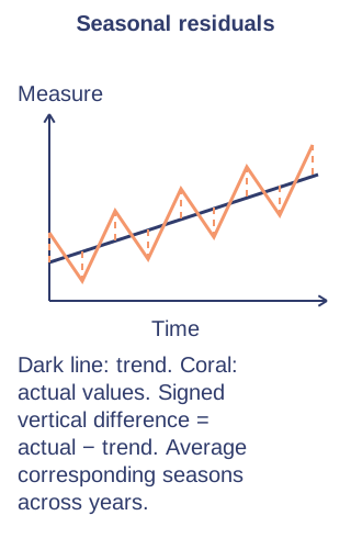
Mean seasonal effect — In an additive model calculate actual minus trend for matching times, then average these deviations for each season across years. Effects should balance around zero for a complete cycle; rounding or imperfect trends can require adjustment. Seasonal variation is a difference in the measure's units.
Seasonal prediction — Add a season's mean effect to the projected trend. If trend predicts 120 sales and the winter effect is −18, forecast 102. Explain that the forecast assumes stable trend and seasonal behaviour; unusual events or extrapolation can make it inaccurate.
Weighted index — Multiply each component index by its weight, add the products and divide by total weight. Indices 110 and 130 with weights 3 and 1 give 115. Weights reflect expenditure or importance; an unweighted mean changes the meaning of the basket.
Chain-based index — Each link compares a period with the preceding period. Multiply link factors to obtain overall change: links 110 then 120 give factor 1.1×1.2=1.32 and overall index 132 from the original base. Do not add the percentage increases.
Standardisation — Follow any supplied rate-standardisation formula and identify its output and denominator. Applying group-specific rates to a common standard population can make comparisons fairer when age structures differ. Do not confuse a predicted count from a rate with a rate per thousand; report the formula's stated units.
Test yourself
30 questions · Sets of 10 from the selected tier. For fractions, use / when typing; for powers, use superscripts or ^. Follow each question's answer format. These quick checks support revision; practise full written solutions, graph constructions and enquiries too.
Mind map
Use the branches to recall the ideas and explain their connections. Check the revision notes for the full detail.
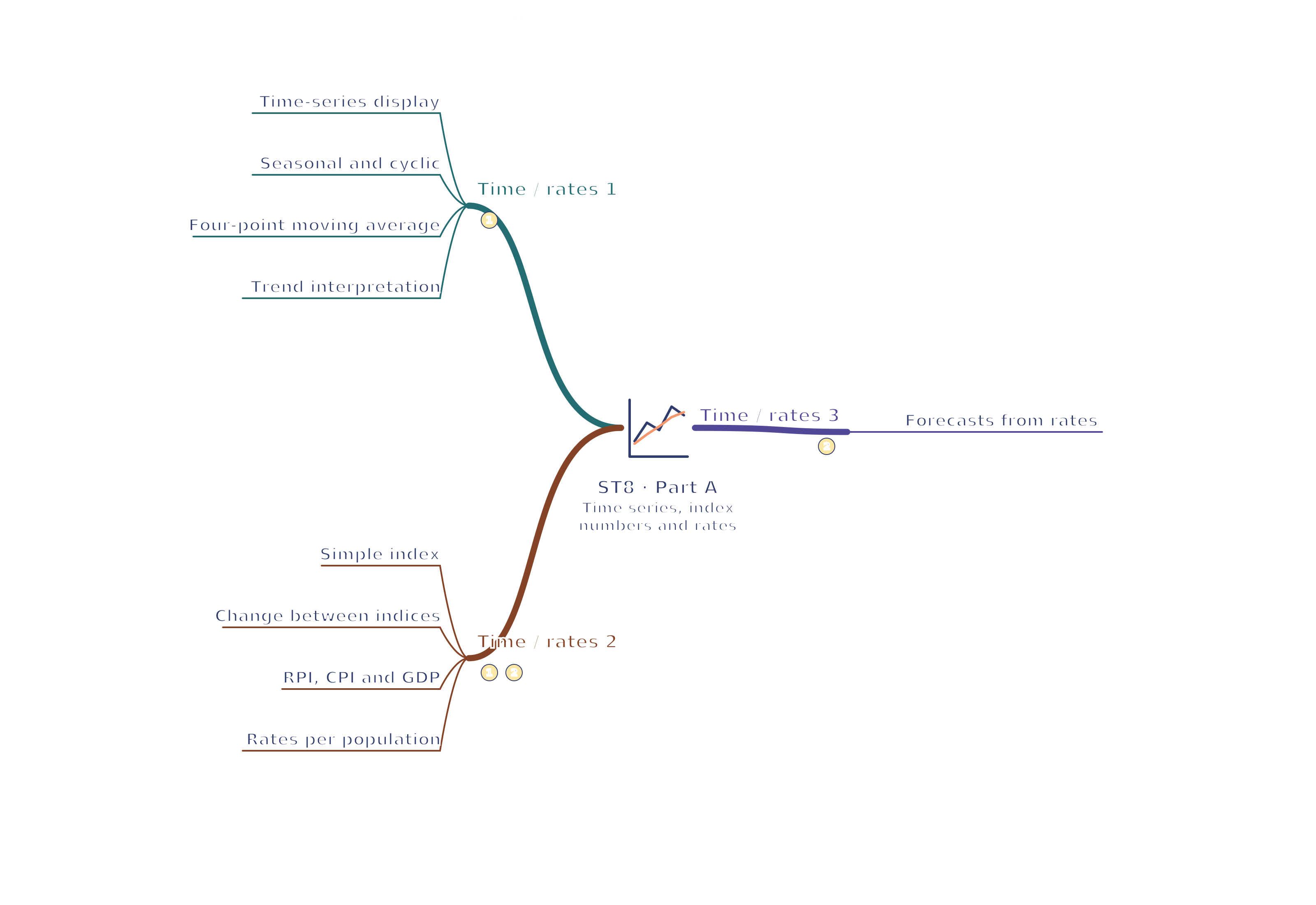
ST8 · Time / rates 1 / Time / rates 2 / Time / rates 3
View ST8 · Time / rates 1 / Time / rates 2 / Time / rates 3 mind mapOpen the full-size map to zoom. Download the PDF to print on A4 or enlarge to A3.
Time-series display: Time on x; separate trend from noise.
Seasonal and cyclic: Seasonal calendar pattern; cycles less fixed.
Four-point moving average: Average successive fours at half-time positions.
Trend interpretation: Smoothing helps show underlying change.
Time / rates 2
Simple index: Base 100; index expresses relative change.
Change between indices: Percentage change uses the earlier denominator.
RPI, CPI and GDP: Check indicator, basket, base and price adjustment.
Rates per population: Standardise counts using the relevant population.
Time / rates 3
Forecasts from rates: Rate-based predictions depend on appropriate populations.
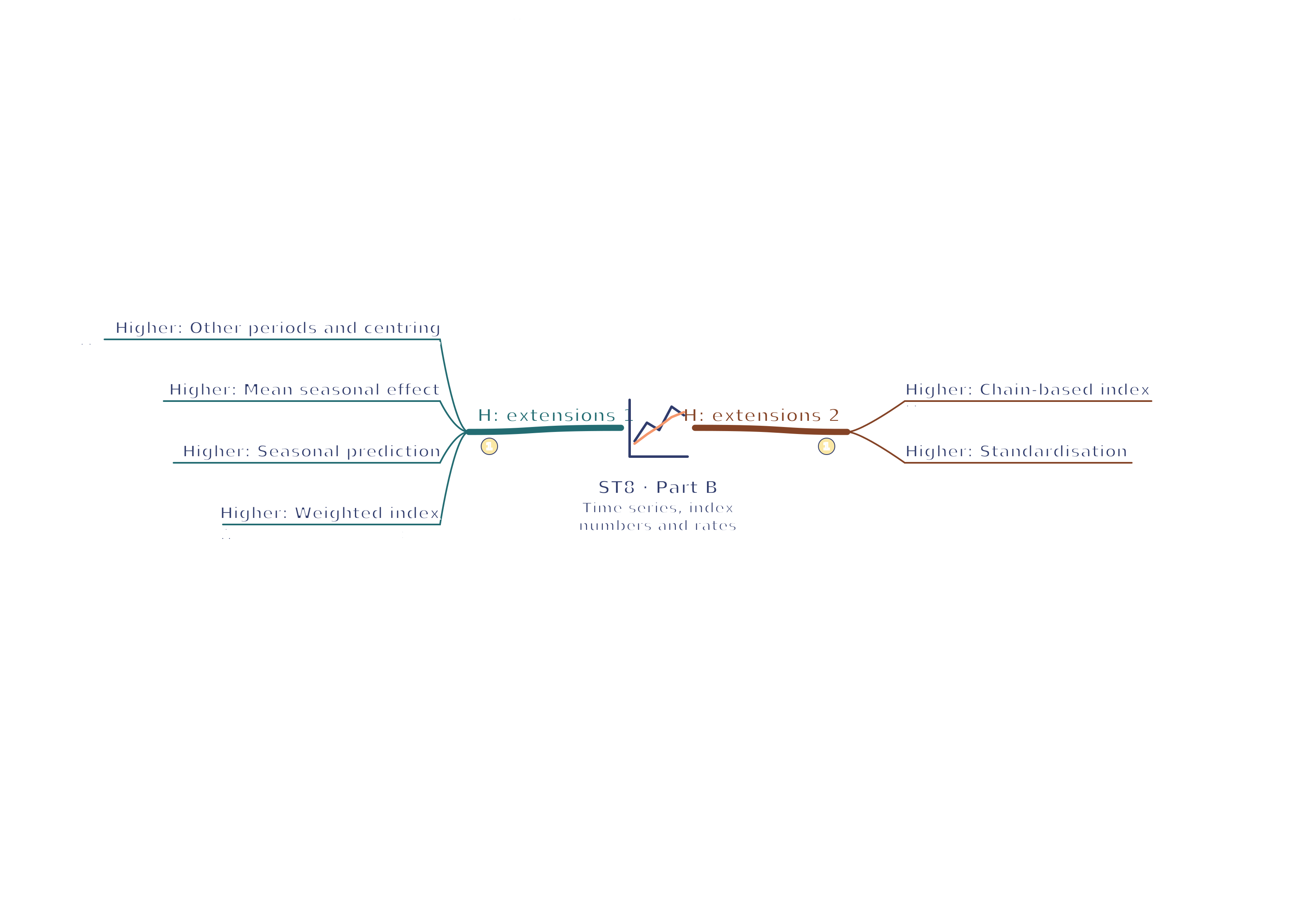
H: extensions 1
Higher: Other periods and centring: Match period; centre even moving averages if needed.
Higher: Mean seasonal effect: Average actual − trend for each season.
Higher: Seasonal prediction: Forecast = trend + mean seasonal effect.
Higher: Weighted index: Weighted index = ΣwI ÷ Σw.
H: extensions 2
Higher: Chain-based index: Multiply link factors across successive periods.
Higher: Standardisation: Common population basis improves rate comparisons.
Connections
Time / rates 1 → Time / rates 2: A smoothed time trend and relative indices describe changes from an explicit reference.
Time / rates 2 → Time / rates 3: Population rates and stated time periods provide the basis for expected-count forecasts.
Part connections
ST8 · Time / rates 1 / Time / rates 2 / Time / rates 3: Time / rates 1 → Time / rates 2 — A smoothed time trend and relative indices describe changes from an explicit reference.
ST8 · Time / rates 1 / Time / rates 2 / Time / rates 3: Time / rates 2 → Time / rates 3 — Population rates and stated time periods provide the basis for expected-count forecasts.
ST8 · H: extensions 1 / H: extensions 2: H: extensions 1 → H: extensions 2 — Additive seasonal forecasts and chain indices use distinct models whose assumptions must be checked.
 Mr Kidman's Classroom