Explain the methods, show your working and interpret results in context.
Foundation shows shared notes and questions. Higher includes the labelled extensions. Maps and checklist downloads include labelled Higher content; the worksheet generator filters individual goals.
Revise the key ideas
Typical values
Arithmetic mean — Add every value then divide by the number of values. For 2, 4 and 9 minutes the mean is 5 minutes. The result need not be an observed value. Show the sum and count and keep unrounded intermediate values for further calculation.
Median — Order the data; the median is the middle value, or mean of the two middle values for an even count. For 3, 4, 8 and 11 it is 6. Ordering is essential; the middle value in the original recording order is not generally the median.
Mode and modal class — The mode is the most frequent value or category; there can be several tied modes or no unique mode. A modal class is the interval with greatest frequency, not its midpoint. Clothing sizes often suit a mode because a non-existent average size may be unhelpful.
Frequency-table mean — Multiply each value x by its frequency f, sum fx and divide by total frequency: mean = Σfx / Σf. Values 2 and 5 with frequencies 3 and 2 give total 16 and count 5, so mean 3.2. Do not divide by the number of rows.Frequency-weighted arithmetic mean. Original illustrative diagram; numerical datasets are fictional worked examples.Enlarge diagram
Grouped mean estimate — Use each class midpoint as a representative value, then calculate Σfm / Σf. Classes 0–10 and 10–20 with frequencies 2 and 3 give (2×5 + 3×15)/5 = 11. This estimates the mean because positions inside classes are unknown.
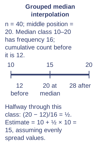
Grouped median — Find the middle observation's cumulative position and identify its class. Estimate its position using a cumulative-frequency graph or linear interpolation. Foundation calculations use equal-width classes. The class midpoint is not automatically the median when the cumulative position is off-centre.
Choose an average — The median resists a few extreme observations and suits skewed income or waiting-time data; the mean uses all measurements and suits later SD comparisons. The mode handles categories. Explain the choice for the data and purpose instead of always claiming one average is best.
Compare centres — Say which group has a higher typical value, quote both appropriate averages and interpret the difference with units. Use comparable definitions and collection periods. A difference between sample means is evidence to discuss, not proof that every member differs or that one factor caused it.
Changes to data — Adding a value above the current mean raises it; removing a below-mean value also raises it. Recalculate the total and count rather than averaging old and new means equally. The median and mode may stay unchanged or change depending on positions and frequencies.
Transformations — Adding c to every numerical observation adds c to mean and median; multiplying by positive k multiplies them by k. Numerical modes transform likewise. A unit conversion needs the same rule for all data; changing only some records creates a different dataset.
Median interpolation — For grouped continuous data use L + ((n/2 − cumulative frequency before)/class frequency) × width. With n=40, L=10, previous total 12, class frequency 16 and width 10, the median estimate is 15. Assume an even spread within the class and state the estimate.
Higher — weighted and geometric averages
Weighted mean — A weighted mean is Σwx / Σw, where weights reflect importance or group sizes. Scores 60 and 80 weighted 1 and 3 give 75. To combine group means, use group sizes as weights; an unweighted average of means only works for equally sized groups.
Geometric mean — For positive values, geometric mean = nth root of their product. For growth factors 1.10 and 1.21 it is √1.331 ≈ 1.15369, giving about 15.37% per period. Average multiplying factors, not percentage numbers; the factors' product must be preserved.
Unequal-width grouped averages — Higher grouped mean and median calculations can use unequal class widths. Use each class's own midpoint in a mean estimate and the actual median class width for interpolation. Do not substitute one standard width for every class or use density in place of frequency in the mean formula.
Test yourself
30 questions · Sets of 10 from the selected tier. For fractions, use / when typing; for powers, use superscripts or ^. Follow each question's answer format. These quick checks support revision; practise full written solutions, graph constructions and enquiries too.
Mind map
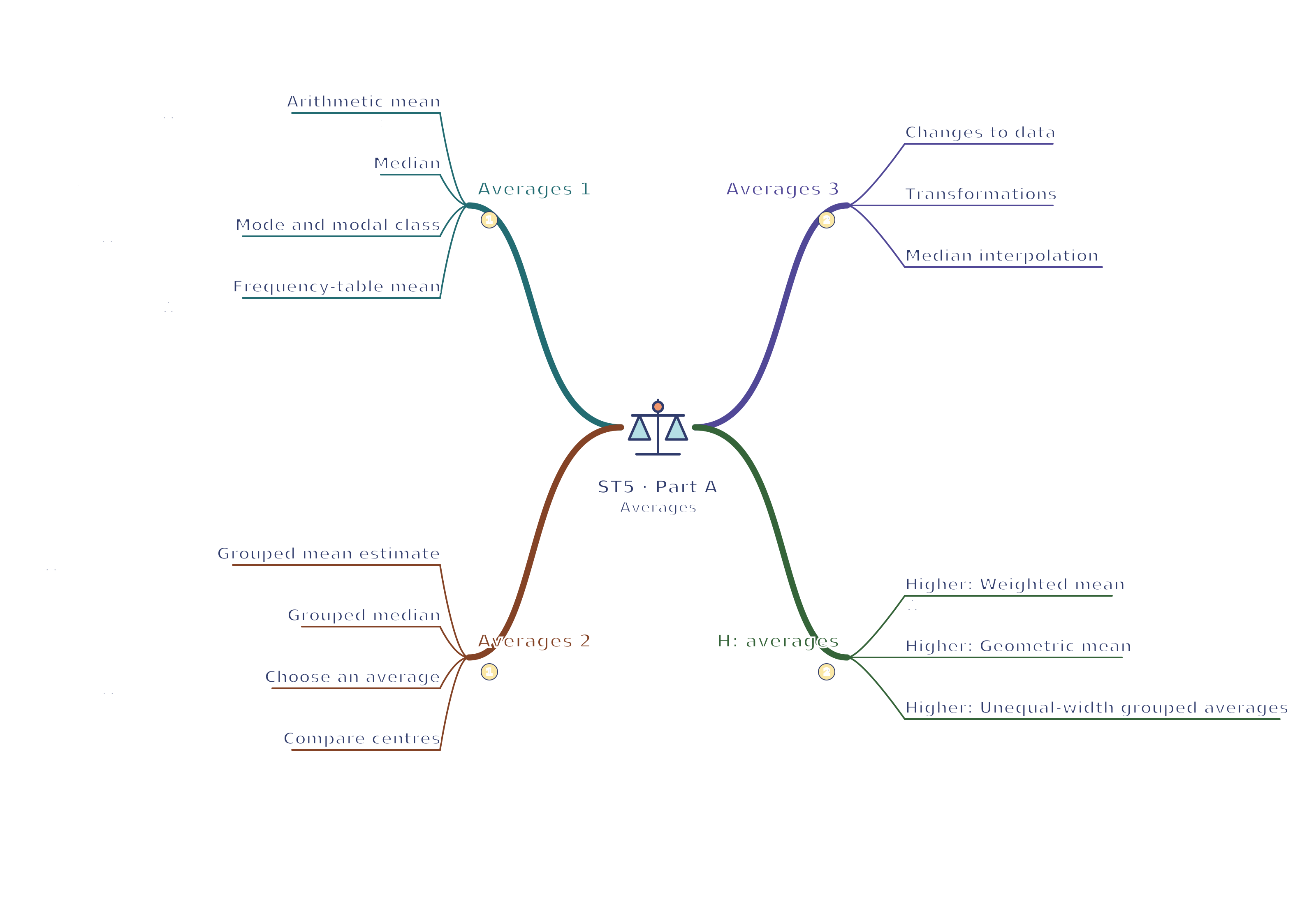
Use the branches to recall the ideas and explain their connections. Check the revision notes for the full detail.
View ST5 · Averages 1 / Averages 2 / Averages 3 / H: averages mind mapOpen the full-size map to zoom. Download the PDF to print on A4 or enlarge to A3.
Arithmetic mean: Mean uses all values: total ÷ count.
Median: Sort first; average two middle values if needed.
Mode and modal class: Most frequent value or class, including ties.
Frequency-table mean: Weight each value by its frequency.
Averages 2
Grouped mean estimate: Midpoints approximate unknown values in classes.
Grouped median: Identify class; interpolate its cumulative position.
Choose an average: Match average to shape, type and purpose.
Compare centres: Compare matching summaries with units and context.
Averages 3
Changes to data: Update total and count; other averages need inspection.
Transformations: Apply consistent translations and positive scaling.
Median interpolation: Interpolate a cumulative position within its class.
H: averages
Higher: Weighted mean: Weighted total divided by total weight.
Higher: Geometric mean: Root of product for repeated multiplicative change.
Higher: Unequal-width grouped averages: Use each actual midpoint and median-class width.
Connections
Averages 1 → Averages 2: Frequency weighting and grouped estimates retain different amounts of exact information about the centre.
Averages 3 → H: averages: Grouped interpolation uses the median class width; Higher also permits unequal class widths.
Part connections
ST5 · Averages 1 / Averages 2 / Averages 3 / H: averages: Averages 1 → Averages 2 — Frequency weighting and grouped estimates retain different amounts of exact information about the centre.
ST5 · Averages 1 / Averages 2 / Averages 3 / H: averages: Averages 3 → H: averages — Grouped interpolation uses the median class width; Higher also permits unequal class widths.
 Mr Kidman's Classroom