Explain the methods, show your working and interpret results in context.
Foundation shows shared notes and questions. Higher includes the labelled extensions. Maps and checklist downloads include labelled Higher content; the worksheet generator filters individual goals.
Revise the key ideas
Binomial models
Conditions — A binomial model counts successes in a fixed number n of independent trials, each with two defined outcomes and constant success probability p. Success is the named event, not necessarily something desirable. Sampling without replacement from a small finite group usually violates independence and constant p.
Notation and support — X ∼ B(n,p) describes a count taking integer values 0 to n. For X∼B(5,0.2), five trials each have success probability 0.2. Edexcel calculations use n no larger than 10; a continuous measurement itself is not a binomial count.
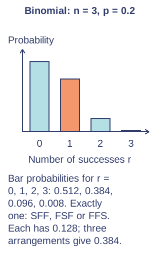
One sequence — A particular sequence of r successes and n−r failures has probability pʳ(1−p)ⁿ⁻ʳ. With n=3 and p=0.2, sequence SFF has probability 0.2×0.8²=0.128. Other sequences with one success have the same probability but are separate outcomes.
Exactly r successes — Multiply the single-sequence probability by the number of arrangements: P(X=r)=C(n,r)pʳ(1−p)ⁿ⁻ʳ. For n=3, r=1 and p=0.2, three arrangements give 0.384. Combinations can be found using a calculator, Pascal's triangle or systematic paths.
At most and at least — At most two means sum P(0), P(1), P(2); at least two means sum from 2 through n or subtract P(0)+P(1) from 1. Check calculator cumulative functions include the boundary required by the wording. Strictly more than two starts at three.
Binomial mean — Expected successes are np. For B(8,0.25), the mean is 2; individual runs can give 0 through 8 successes. An expected frequency among repeated groups uses the probability of the specified count, which differs from the expected successes inside one group.
Check a model — Compare observed frequencies with expected probabilities multiplied by the number of groups. Large persistent discrepancies may suggest varying p, dependence, selection bias or recording problems. Ordinary random variation also gives differences; describe possible bias without formal significance testing.
Normal models and intervals
Normal shape — A normal distribution is continuous, symmetric and bell-shaped with mean, median and mode equal. Mean μ locates the centre and SD σ controls spread. Examine real data before adopting it; a symmetric flat or bimodal shape is not normal merely because it is symmetric.
Normal notation — X∼N(μ,σ²) gives the variance as the second parameter. N(50,16) therefore has mean 50 and SD 4, not 16. The ideal curve has tails extending indefinitely; real measurements and limited samples need contextual checking.
One SD — Approximately 68% lies between μ−σ and μ+σ, about 34% on each side of the mean within that interval. For mean 100 and SD 10, about 68% lies from 90 to 110. This is an approximate model statement, not an exact guarantee in every sample.Normal intervals use standard deviation. Original illustrative diagram; numerical datasets are fictional worked examples.Enlarge diagram
Two SDs — Approximately 95% lies within μ±2σ, leaving about 5% outside, split into about 2.5% in each tail by symmetry. For mean 100 and SD 10 the interval is 80–120. Do not put all 5% in one tail.
Three SDs — Values farther than three SDs from the mean are very unusual under a normal model; approximately 99.7% lies inside. With mean 50 and SD 4, values outside 38–62 are unusual. An unusual genuine observation is still possible and need not be removed.
Regions and expected counts — Use symmetry and subtraction between stated intervals. The share between one and two SDs above the mean is approximately (95−68)/2 =13.5%; among 200 comparable observations expect about 27 there. Normal tables are not required; use the supplied proportions with their stated precision.
Suitability and judgement — A normal model may suit continuous data that cluster in a roughly symmetric bell shape. Strong skew, truncation or distinct subgroups can make it misleading. Explain assumptions and limitations before predicting proportions; model fit and statistical enquiry need more than a single numerical answer.
Test yourself
30 questions · Sets of 10 from the selected tier. For fractions, use / when typing; for powers, use superscripts or ^. Follow each question's answer format. These quick checks support revision; practise full written solutions, graph constructions and enquiries too.
Mind map
Use the branches to recall the ideas and explain their connections. Check the revision notes for the full detail.
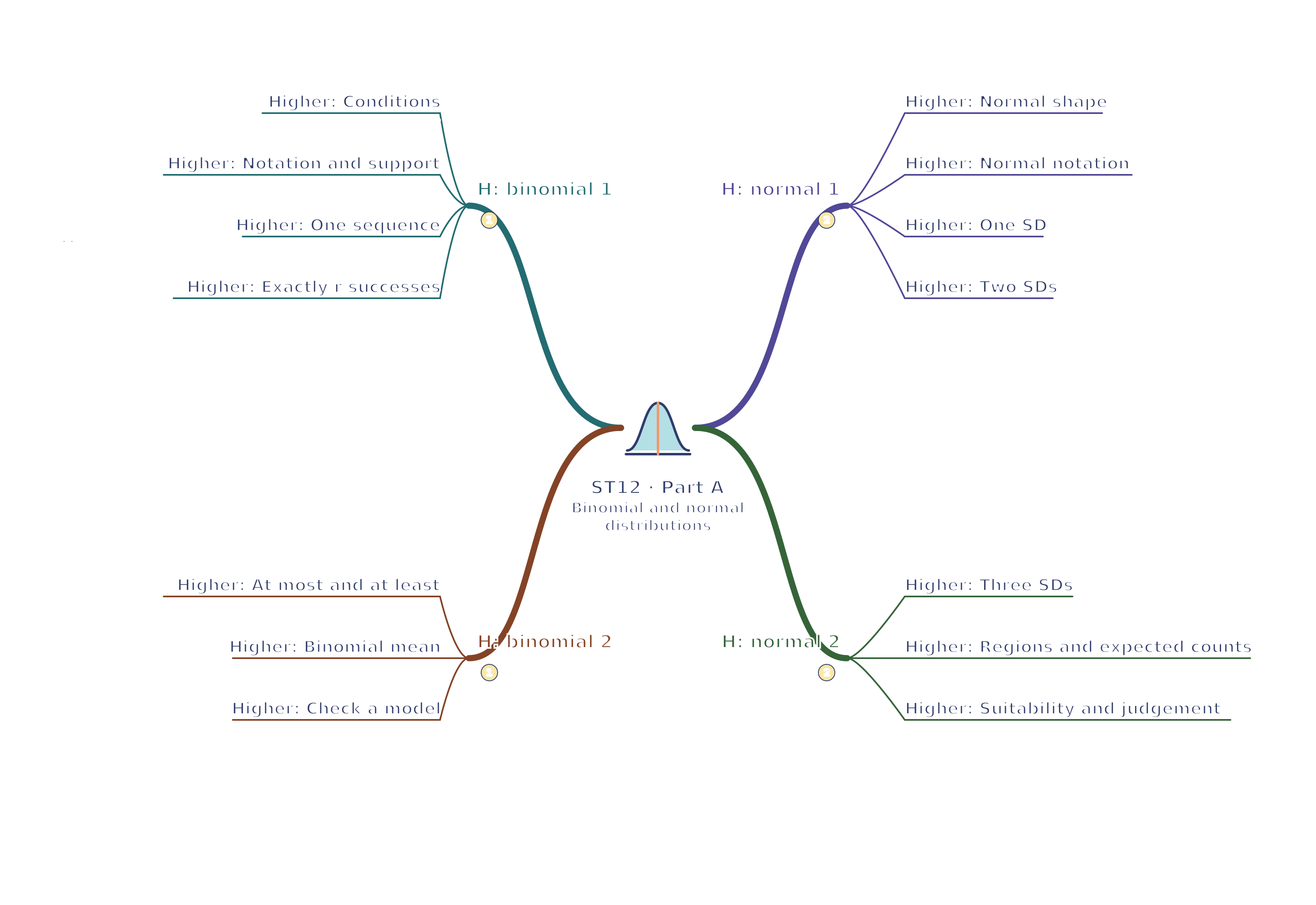
ST12 · H: binomial 1 / H: binomial 2 / H: normal 1 / H: normal 2
View ST12 · H: binomial 1 / H: binomial 2 / H: normal 1 / H: normal 2 mind mapOpen the full-size map to zoom. Download the PDF to print on A4 or enlarge to A3.
Higher: Conditions: Fixed n; independent two-outcome trials; constant p.
Higher: Notation and support: Binomial counts are integers from 0 to n.
Higher: One sequence: Multiply success and failure probabilities for one path.
Higher: Exactly r successes: Count arrangements then multiply path probability.
H: binomial 2
Higher: At most and at least: Inequality words determine included integer counts.
Higher: Binomial mean: np is average successes per group, not certainty.
Higher: Check a model: Compare observed with expected; consider model conditions.
H: normal 1
Higher: Normal shape: Continuous symmetric bell shape; centre measures coincide.
Higher: Normal notation: Second normal parameter is variance; take its square root.
Higher: One SD: Approximately 68% within one SD.
Higher: Two SDs: Approximately 95% within two SDs; tails 2.5% each.
H: normal 2
Higher: Three SDs: Beyond three SDs is very unusual, not impossible.
Higher: Regions and expected counts: Symmetry and subtraction locate model regions.
Higher: Suitability and judgement: Check variable, shape and context before modelling.
Connections
H: binomial 1 → H: binomial 2: Binomial conditions justify success-count probabilities used for expectations and model checks.
H: normal 1 → H: normal 2: The normal centre and SD define intervals whose approximate proportions support region estimates.
Part connections
ST12 · H: binomial 1 / H: binomial 2 / H: normal 1 / H: normal 2: H: binomial 1 → H: binomial 2 — Binomial conditions justify success-count probabilities used for expectations and model checks.
ST12 · H: binomial 1 / H: binomial 2 / H: normal 1 / H: normal 2: H: normal 1 → H: normal 2 — The normal centre and SD define intervals whose approximate proportions support region estimates.
 Mr Kidman's Classroom