Explain the methods, show your working and interpret results in context.
Foundation shows shared notes and questions. Higher includes the labelled extensions. Maps and checklist downloads include labelled Higher content; the worksheet generator filters individual goals.
Revise the key ideas
Likelihood and experimental evidence
Probability scale — Probability lies between 0 and 1: 0 is impossible, 1 certain and 0.5 an even chance. Convert consistently between fractions, decimals and percentages. Likely does not mean guaranteed; a single outcome cannot show whether an assigned probability was correct.
Theoretical models — Count favourable outcomes / all outcomes only when outcomes are equally likely. A fair six-sided die gives P(even)=3/6=1/2. A biased spinner's labelled sections may not have equal probabilities, so counting labels alone is insufficient.
Complement — An event and its complement exhaust the possibilities without overlap, so P(not A)=1−P(A). If probability of a late bus is 0.18, probability of not late is 0.82. Define the event carefully: not winning can include both drawing and losing.
Relative frequency — Estimate probability as observed event count / trial count. If 28 of 80 deliveries are late, estimated probability is 0.35. Keep a consistent event definition and report the number of trials; observed proportions vary between samples.
Expected frequency — Multiply probability by the number of trials: E=np. With p=0.3 in 200 trials expect 60 events on average. An expectation is not a guaranteed realised count, and it need not be a whole number when describing the average of many repeated trials.
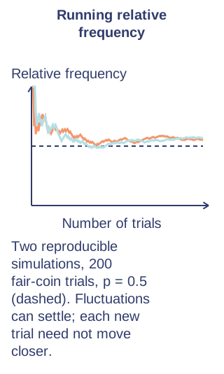
Long-run behaviour — Under suitable random repeated trials with a stable probability, relative frequency tends to settle nearer that probability as trial count grows. It does not move closer after every extra trial, and past failures do not make an independent future success compulsory.
Assess possible bias — Compare observed counts with expected values, taking trial size and ordinary variation into account. A die showing six twice in twelve rolls is compatible with many models; a substantial persistent discrepancy across many trials is stronger reason to question fairness or collection. Formal significance tests are not required.
Simulation — Use random digits or calculator outcomes with probabilities matching the model. To simulate probability 0.3 using digits 0–9, designate three digits as success. State independence assumptions and run enough repetitions; a poor mapping biases the simulation before it begins.
Absolute and relative risk
Absolute risk — Risk is a probability of a specified outcome in a defined group and period. If 4 of 200 items fail, absolute risk is 0.02 or 2%. State what failure means and the denominator; a count alone cannot compare groups of different sizes fairly.
Relative risk — Divide risk in group A by risk in reference group B. Risks 0.06 and 0.03 give relative risk 2: A's risk is twice B's. Specify the order; reversing it gives 0.5, and a zero reference risk makes this ratio undefined.Compare risks using a common denominator. Original illustrative diagram; numerical datasets are fictional worked examples.Enlarge diagram
Risk difference — Subtract absolute risks to show the probability difference. An increase from 1% to 2% is one percentage point, a 100% relative increase and a relative risk of 2. Give the baseline so a striking relative statement does not hide a small absolute difference.
Expected groups — A risk of 0.015 corresponds to about 15 outcomes per 1000 comparable cases. Present both groups on the same denominator to communicate clearly. Observational risk differences can be confounded; do not automatically attribute them to the named exposure or intervention.
Test yourself
30 questions · Sets of 10 from the selected tier. For fractions, use / when typing; for powers, use superscripts or ^. Follow each question's answer format. These quick checks support revision; practise full written solutions, graph constructions and enquiries too.
Mind map
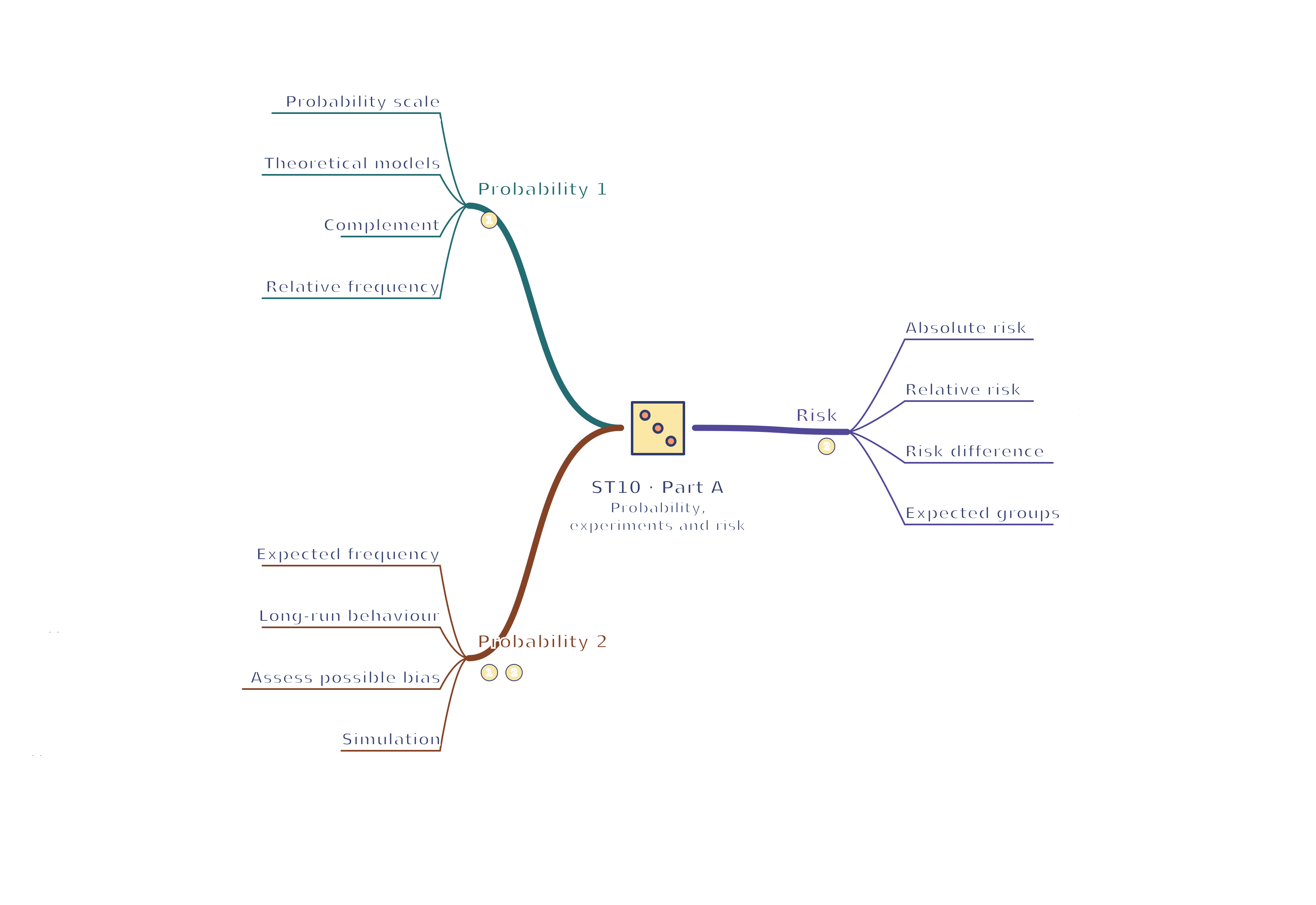
Use the branches to recall the ideas and explain their connections. Check the revision notes for the full detail.
ST10 · Probability 1 / Probability 2 / Risk
View ST10 · Probability 1 / Probability 2 / Risk mind mapOpen the full-size map to zoom. Download the PDF to print on A4 or enlarge to A3.
Long-run behaviour: More trials stabilise estimates without guaranteed convergence steps.
Assess possible bias: Persistent discrepancies need investigation, not instant proof.
Simulation: Map random outcomes to the intended probabilities.
Risk
Absolute risk: Risk = events ÷ relevant group total.
Relative risk: Relative risk = A risk ÷ reference risk.
Risk difference: Absolute difference differs from relative percentage change.
Expected groups: Common denominators make risk comparisons clearer.
Connections
Probability 1 → Probability 2: Theoretical probabilities and relative frequencies determine expectations compared with repeated trials.
Probability 2 → Risk: Expected event counts put absolute and relative risks on comparable group denominators.
Part connections
ST10 · Probability 1 / Probability 2 / Risk: Probability 1 → Probability 2 — Theoretical probabilities and relative frequencies determine expectations compared with repeated trials.
ST10 · Probability 1 / Probability 2 / Risk: Probability 2 → Risk — Expected event counts put absolute and relative risks on comparable group denominators.
 Mr Kidman's Classroom